Estimate tree growth rates from FIADB

Computes estimates of average annual DBH, basal area, height, and net volume growth rates for individual stems, along with average annual basal area and net volume growth per acre. Only stems 5 inches DBH or greater are included in estimates. Estimates can be produced for regions defined within the FIA Database (e.g. counties), at the plot level, or within user-defined areal units. Options to group estimates by species, size class, and other variables defined in the FIADB. If multiple reporting years (EVALIDs) are included in the data, estimates will be output as a time series. If multiple states are represented by the data, estimates will be output for the full region (all area combined), unless specified otherwise (e.g. grpBy = STATECD).

Usage

vitalRates(db, grpBy = NULL, polys = NULL, returnSpatial = FALSE, bySpecies = FALSE,
           bySizeClass = FALSE, landType = 'forest', treeType = 'all',
           method = 'TI', lambda = .5, treeDomain = NULL,
           areaDomain = NULL, totals = FALSE, variance = FALSE,
           byPlot = FALSE, treeList = FALSE, nCores = 1)

Arguments

db: FIA.Database or Remote.FIA.Database object produced from readFIA() or getFIA(). If a Remote.FIA.Database, data will be read in and processed state-by-state to conserve RAM (see details for an example).
grpBy: variables from PLOT, COND, or TREE tables to group estimates by (NOT quoted). Multiple grouping variables should be combined with c(), and grouping will occur heirarchically. For example, to produce seperate estimates for each ownership group within methods of stand regeneration, specify c(STDORGCD, OWNGRPCD).
polys: sp or sf Polygon/MultiPolgyon object; Areal units to bin data for estimation. Separate estimates will be produced for region encompassed by each areal unit. FIA plot locations will be reprojected to match projection of polys object.
returnSpatial: logical; if TRUE, merge population estimates with polys and return as sf multipolygon object. When byPlot = TRUE, return plot-level estimates as sf spatial points.
bySpecies: logical; if TRUE, returns estimates grouped by species.
bySizeClass: logical; if TRUE, returns estimates grouped by size class (2-inch intervals, see makeClasses() to compute different size class intervals).
landType: character ("forest" or "timber"); Type of land which estimates will be produced for. Timberland is a subset of forestland (default) which has high site potential and non-reserve status (see details).
treeType: character ("all", "live", or "gs"); Type of tree which estimates will be produced for. See details for more info.
method: character; design-based estimator to use. One of: "TI" (temporally indifferent, default), "annual" (annual), "SMA" (simple moving average), "LMA" (linear moving average), or "EMA" (exponential moving average). See Stanke et al 2020 for a complete description of these estimators.
lambda: numeric (0,1); if method = 'EMA', the decay parameter used to define weighting scheme for annual panels. Low values place higher weight on more recent panels, and vice versa. Specify a vector of values to compute estimates using mulitple weighting schemes, and use plotFIA() with grp set to lambda to produce moving average ribbon plots. See Stanke et al 2020 for examples.
treeDomain: logical predicates defined in terms of the variables in PLOT, TREE, and/or COND tables. Used to define the type of trees for which estimates will be produced (e.g. DBH greater than 20 inches: DIA > 20, Dominant/Co-dominant crowns only: CCLCD %in% c(2,3). Multiple conditions are combined with & (and) or | (or). Only trees where the condition evaluates to TRUE are used in producing estimates. Should NOT be quoted.
areaDomain: logical predicates defined in terms of the variables in PLOT and/or COND tables. Used to define the area for which estimates will be produced (e.g. within 1 mile of improved road: RDDISTCD %in% c(1:6), Hard maple/basswood forest type: FORTYPCD == 805. Multiple conditions are combined with & (and) or | (or). Only plots within areas where the condition evaluates to TRUE are used in producing estimates. Should NOT be quoted.
totals: logical; if TRUE, return total population estimates (e.g. total area) along with ratio estimates (e.g. mean trees per acre).
variance: logical; if TRUE, return estimated variance (VAR) and sample size (N). If FALSE, return 'sampling error' (SE) as returned by EVALIDator. Note: sampling error cannot be used to construct confidence intervals.
byPlot: logical; if TRUE, returns estimates for individual plot locations instead of population estimates.
treeList: logical; if TRUE, returns tree-level summaries intended for subsequent use with customPSE()

nCores: numeric; number of cores to use for parallel implementation. Check available cores using detectCores. Default = 1, serial processing.

Details

Estimation Details

Estimation of forest variables follows the procedures documented in Bechtold and Patterson (2005) and Stanke et al 2020.

Average annual diameter, basal area, height, and net volume growth of a stem is computed using a sample-based ratio of means estimator of total diameter (basal area, height, net volume) growth / total trees, and average annual basal area and net volume growth per acre is computed as total basal area (net volume) growth / total area. All estimates are returned as average annual rates. Only conditions which were forest in time 1 and in time 2 are included in estimates (excluding converted stands). Only stems 5 inches DBH or greater are included in estimates.

When treeType = 'all' (default), estimates are of net growth rates (including recruitment and mortality), and hence they may attain a negative value. Negative growth estimates most likely indicate a substantial change in an attribute of the tree or area between time 1 and time 2, which caused the attribute to decrease. Implementation of the growth accounting method allows us to more accurately represent shifts in forest attributes (biomass) between classified groups (size classes) over time. Alternatively, when treeType = 'live', growth rates are calculated using only trees that were alive at both plot visits and give a more realistic representation of individual tree growth.

Users may specify alternatives to the 'Temporally Indifferent' estimator using the method argument. Alternative design-based estimators include the annual estimator ("ANNUAL"; annual panels, or estimates from plots measured in the same year), simple moving average ("SMA"; combines annual panels with equal weight), linear moving average ("LMA"; combine annual panels with weights that decay linearly with time since measurement), and exponential moving average ("EMA"; combine annual panels with weights that decay exponentially with time since measurement). The "best" estimator depends entirely on user-objectives, see Stanke et al 2020 for a complete description of these estimators and tradeoffs between precision and temporal specificity.

When byPlot = FALSE (i.e., population estimates are returned), the "YEAR" column in the resulting dataframe indicates the final year of the inventory cycle that estimates are produced for. For example, an estimate of current forest area (e.g., 2018) may draw on data collected from 2008-2018, and "YEAR" will be listed as 2018 (consistent with EVALIDator). However, when byPlot = TRUE (i.e., plot-level estimates returned), the "YEAR" column denotes the year that each plot was measured (MEASYEAR), which may differ slightly from its associated inventory year (INVYR).

Stratified random sampling techniques are most often employed to compute estimates in recent inventories, although double sampling and simple random sampling may be employed for early inventories. Estimates are adjusted for non-response bias by assuming attributes of non-response plot locations to be equal to the mean of other plots included within thier respective stratum or population.

Working with "Big Data"

If FIA data are too large to hold in memory (e.g., R throws the "cannot allocate vector of size ..." errors), use larger-than-RAM options. See documentation of link{readFIA} for examples of how to set up a Remote.FIA.Database. As a reference, we have used rFIA's larger-than-RAM methods to estimate forest variables using the entire FIA Database (~50GB) on a standard desktop computer with 16GB of RAM. Check out our website for more details and examples.

Easy, efficient parallelization is implemented with the parallel package. Users must only specify the nCores argument with a value greater than 1 in order to implement parallel processing on their machines. Parallel implementation is achieved using a snow type cluster on any Windows OS, and with multicore forking on any Unix OS (Linux, Mac). Implementing parallel processing may substantially decrease free memory during processing, particularly on Windows OS. Thus, users should be cautious when running in parallel, and consider implementing serial processing for this task if computational resources are limited (nCores = 1).

Definition of forestland

Forest land must have at least 10-percent canopy cover by live tally trees of any size, including land that formerly had such tree cover and that will be naturally or artificially regenerated. Forest land includes transition zones, such as areas between heavily forest and non-forested lands that meet the mimium tree canopy cover and forest areas adjacent to urban and built-up lands. The minimum area for classification of forest land is 1 acre in size and 120 feet wide measured stem-to-stem from the outer-most edge. Roadside, streamside, and shelterbelt strips of trees must have a width of at least 120 feet and continuous length of at least 363 feet to qualify as forest land. Tree-covered areas in agricultural production settings, such as fruit orchards, or tree-covered areas in urban settings, such as city parks, are not considered forest land.

Timber land is a subset of forest land that is producing or is capable of producing crops of industrial wood and not withdrawn from timber utilization by statute or administrative regulation. (Note: Areas qualifying as timberland are capable of producing at least 20 cubic feet per acre per year of industrial wood in natural stands. Currently inaccessible and inoperable areas are NOT included).

Value

Dataframe or sf object (if returnSpatial = TRUE). If byPlot = TRUE, values are returned for each plot (PLOT_STATUS_CD = 1 when forest exists at the plot location). All variables with names ending in SE, represent the estimate of sampling error (%) of the variable. When variance = TRUE, variables ending in VAR denote the variance of the variable and N is the total sample size (i.e., including non-zero plots).

YEAR: reporting year associated with estimates
DIA_GROW: estimate of mean annual diameter growth of a stem (inches/ yr)
BA_GROW: estimate of mean annual basal area growth of a stem (sq. ft./ yr)
BAA_GROW: estimate of mean annual basal area growth per acre (sq. ft./ acre/ yr)
NETVOL_GROW: estimate of mean annual net volume growth of a stem (cu. ft./ yr)
NETVOL_GROW_AC: estimate of mean annual net volume growth per acre (cu. ft./ acre/ yr)
SAWVOL_GROW: estimate of mean annual net sawlog volume growth of a stem (MBF / yr)
SAWVOL_GROW_AC: estimate of mean annual net sawlog volume growth per acre (MBF/ acre/ yr)
BIO_GROW: estimate of mean annual aboveground biomass growth of a stem (short tons/ yr)
BIO_GROW_AC: estimate of mean annual aboveground biomass growth per acre (short tons/ acre/ yr)
nPlots_TREE: number of non-zero plots used to compute tree and basal area estimates
nPlots_AREA: number of non-zero plots used to compute land area estimates

References

rFIA website: https://rfia.netlify.app/

FIA Database User Guide: https://research.fs.usda.gov/understory/forest-inventory-and-analysis-database-user-guide-nfi

Bechtold, W.A.; Patterson, P.L., eds. 2005. The Enhanced Forest Inventory and Analysis Program - National Sampling Design and Estimation Procedures. Gen. Tech. Rep. SRS - 80. Asheville, NC: U.S. Department of Agriculture, Forest Service, Southern Research Station. 85 p. https://www.srs.fs.usda.gov/pubs/gtr/gtr_srs080/gtr_srs080.pdf

Stanke, H., Finley, A. O., Weed, A. S., Walters, B. F., & Domke, G. M. (2020). rFIA: An R package for estimation of forest attributes with the US Forest Inventory and Analysis database. Environmental Modelling & Software, 127, 104664.

Author

Hunter Stanke and Andrew Finley

Note

All sampling error estimates (SE) are returned as the "percent coefficient of variation" (standard deviation / mean * 100) for consistency with EVALIDator. IMPORTANT: sampling error cannot be used to construct confidence intervals. Please use variance = TRUE for that (i.e., return variance and sample size instead of sampling error).

Examples

# Load data from the rFIA package
data(fiaRI)
data(countiesRI)

# Most recents subset
fiaRI_mr <- clipFIA(fiaRI)


# Most recent estimates for growing-stock on timber land
vitalRates(db = fiaRI_mr,
           landType = 'timber',
           treeType = 'gs')
#> # A tibble: 1 × 22
#>    YEAR DIA_GROW BA_GROW NETVOL_GROW SAWVOL_GROW BIO_GROW BA_GROW_AC
#>   <dbl>    <dbl>   <dbl>       <dbl>       <dbl>    <dbl>      <dbl>
#> 1  2018   0.0325 0.00690       0.254     0.00131  0.00680      0.957
#> # ℹ 15 more variables: NETVOL_GROW_AC <dbl>, SAWVOL_GROW_AC <dbl>,
#> #   BIO_GROW_AC <dbl>, DIA_GROW_SE <dbl>, BA_GROW_SE <dbl>,
#> #   NETVOL_GROW_SE <dbl>, SAWVOL_GROW_SE <dbl>, BIO_GROW_SE <dbl>,
#> #   BA_GROW_AC_SE <dbl>, NETVOL_GROW_AC_SE <dbl>, SAWVOL_GROW_AC_SE <dbl>,
#> #   BIO_GROW_AC_SE <dbl>, nPlots_TREE <int>, nPlots_AREA <int>, N <int>
# \donttest{

# Same as above but at the plot-level
vitalRates(db = fiaRI_mr,
           landType = 'timber',
           treeType = 'gs',
           byPlot = TRUE)
#> # A tibble: 114 × 14
#>     YEAR pltID       PLT_CN DIA_GROW   BA_GROW NETVOL_GROW SAWVOL_GROW BIO_GROW
#>    <int> <chr>        <dbl>    <dbl>     <dbl>       <dbl>       <dbl>    <dbl>
#>  1  2013 1_44_1_228 1.45e13   0.121    0.0108       0.400     0.000481    23.5 
#>  2  2013 1_44_3_144 1.45e13   0.0683   0.00698      0.189     0.00210      9.45
#>  3  2013 1_44_7_126 2.47e14   0.321    0.0102       0.104     0.00257      9.75
#>  4  2013 1_44_7_169 1.45e13  -0.306   -0.0154      -0.0896   -0.000488   -24.4 
#>  5  2013 1_44_7_177 2.47e14   0.387    0.0164       0.173     0           13.0 
#>  6  2013 1_44_7_229 1.45e13   0.106    0.0151       0.672     0.00311     45.7 
#>  7  2013 1_44_7_245 1.45e13   0.252    0.0327       0.765     0.00398     46.1 
#>  8  2013 1_44_7_306 1.45e13   0.180    0.0304       0.314     0.00432     50.0 
#>  9  2013 1_44_7_341 2.47e14 NaN      NaN          NaN       NaN          NaN   
#> 10  2013 1_44_7_77  1.45e13   0.121    0.00973      0.198     0.000934    12.6 
#> # ℹ 104 more rows
#> # ℹ 6 more variables: BAA_GROW <dbl>, NETVOL_GROW_AC <dbl>,
#> #   SAWVOL_GROW_AC <dbl>, BIO_GROW_AC <dbl>, PREV_TPA <dbl>, PROP_FOREST <dbl>

# Estimates for white pine ( > 12" DBH) on forested mesic sites
vitalRates(fiaRI_mr,
           treeType = 'live',
           treeDomain = SPCD == 129 & DIA > 12, # Species code for white pine
           areaDomain = PHYSCLCD %in% 21:29) # Mesic Physiographic classes
#> # A tibble: 1 × 22
#>    YEAR DIA_GROW BA_GROW NETVOL_GROW SAWVOL_GROW BIO_GROW BA_GROW_AC
#>   <dbl>    <dbl>   <dbl>       <dbl>       <dbl>    <dbl>      <dbl>
#> 1  2018    0.130  0.0261        1.20     0.00470   0.0194      0.208
#> # ℹ 15 more variables: NETVOL_GROW_AC <dbl>, SAWVOL_GROW_AC <dbl>,
#> #   BIO_GROW_AC <dbl>, DIA_GROW_SE <dbl>, BA_GROW_SE <dbl>,
#> #   NETVOL_GROW_SE <dbl>, SAWVOL_GROW_SE <dbl>, BIO_GROW_SE <dbl>,
#> #   BA_GROW_AC_SE <dbl>, NETVOL_GROW_AC_SE <dbl>, SAWVOL_GROW_AC_SE <dbl>,
#> #   BIO_GROW_AC_SE <dbl>, nPlots_TREE <int>, nPlots_AREA <int>, N <int>

# Most recent estimates grouped by stand age on forest land
# Make a categorical variable which represents stand age (grouped by 10 yr intervals)
fiaRI_mr$COND$STAND_AGE <- makeClasses(fiaRI_mr$COND$STDAGE, interval = 10)
vitalRates(db = fiaRI_mr,
           grpBy = STAND_AGE)
#> # A tibble: 11 × 23
#>     YEAR STAND_AGE DIA_GROW BA_GROW NETVOL_GROW SAWVOL_GROW BIO_GROW BA_GROW_AC
#>    <dbl> <chr>        <dbl>   <dbl>       <dbl>       <dbl>    <dbl>      <dbl>
#>  1  2018 [0,10)     1.08    0.0307       0.122    0          0.00722      0.185
#>  2  2018 [20,30)    0.131   0.00815      0.146    0          0.00425      0.196
#>  3  2018 [30,40)    0.244   0.0178       0.361    0.000723   0.0121       3.29 
#>  4  2018 [40,50)    0.220   0.0132       0.253    0.000380   0.00749      2.58 
#>  5  2018 [50,60)    0.0537  0.00843      0.116   -0.0000363  0.00708      1.47 
#>  6  2018 [60,70)    0.0313  0.00598      0.215    0.000236   0.00720      1.24 
#>  7  2018 [70,80)   -0.00306 0.00336      0.124    0.000298   0.00325      0.678
#>  8  2018 [80,90)   -0.0125  0.00326      0.146    0.000530   0.00431      0.585
#>  9  2018 [90,100)  -0.00871 0.00441      0.0735   0.000443   0.00339      0.677
#> 10  2018 [100,110)  0.0268  0.00750      0.386    0.00153    0.00800      1.09 
#> 11  2018 [110,120]  0.0255  0.0107       0.0374   0.0000806  0.00726      1.67 
#> # ℹ 15 more variables: NETVOL_GROW_AC <dbl>, SAWVOL_GROW_AC <dbl>,
#> #   BIO_GROW_AC <dbl>, DIA_GROW_SE <dbl>, BA_GROW_SE <dbl>,
#> #   NETVOL_GROW_SE <dbl>, SAWVOL_GROW_SE <dbl>, BIO_GROW_SE <dbl>,
#> #   BA_GROW_AC_SE <dbl>, NETVOL_GROW_AC_SE <dbl>, SAWVOL_GROW_AC_SE <dbl>,
#> #   BIO_GROW_AC_SE <dbl>, nPlots_TREE <int>, nPlots_AREA <int>, N <int>

# Most recent estimates for live stems on forest land by species
vitalRates(db = fiaRI_mr,
           landType = 'forest',
           bySpecies = TRUE)
#> # A tibble: 41 × 25
#>     YEAR  SPCD COMMON_NAME         SCIENTIFIC_NAME DIA_GROW  BA_GROW NETVOL_GROW
#>    <dbl> <dbl> <chr>               <chr>              <dbl>    <dbl>       <dbl>
#>  1  2018    12 balsam fir          Abies balsamea   -0.333  -0.00741     -0.0135
#>  2  2018    43 Atlantic white-ced… Chamaecyparis …   0.199   0.0242       0.402 
#>  3  2018    68 eastern redcedar    Juniperus virg…   0.112   0.00480      0.0613
#>  4  2018   126 pitch pine          Pinus rigida     -0.0186  0.00233      0.145 
#>  5  2018   129 eastern white pine  Pinus strobus     0.0617  0.0111       0.479 
#>  6  2018   130 Scotch pine         Pinus sylvestr…   0.205   0.0124       0.278 
#>  7  2018   261 eastern hemlock     Tsuga canadens…   0.128   0.00526      0.0926
#>  8  2018   313 boxelder            Acer negundo      0.25    0.0303       0.684 
#>  9  2018   316 red maple           Acer rubrum       0.0311  0.00343      0.0398
#> 10  2018   317 silver maple        Acer saccharin…   0.505   0.0318      -0.116 
#> # ℹ 31 more rows
#> # ℹ 18 more variables: SAWVOL_GROW <dbl>, BIO_GROW <dbl>, BA_GROW_AC <dbl>,
#> #   NETVOL_GROW_AC <dbl>, SAWVOL_GROW_AC <dbl>, BIO_GROW_AC <dbl>,
#> #   DIA_GROW_SE <dbl>, BA_GROW_SE <dbl>, NETVOL_GROW_SE <dbl>,
#> #   SAWVOL_GROW_SE <dbl>, BIO_GROW_SE <dbl>, BA_GROW_AC_SE <dbl>,
#> #   NETVOL_GROW_AC_SE <dbl>, SAWVOL_GROW_AC_SE <dbl>, BIO_GROW_AC_SE <dbl>,
#> #   nPlots_TREE <int>, nPlots_AREA <int>, N <int>

# Same as above, but implemented in parallel (much quicker)
parallel::detectCores(logical = FALSE) # 4 cores available, we will take 2
#> [1] 16
vitalRates(db = fiaRI_mr,
           landType = 'forest',
           bySpecies = TRUE,
           nCores = 2)
#> # A tibble: 41 × 25
#>     YEAR  SPCD COMMON_NAME         SCIENTIFIC_NAME DIA_GROW  BA_GROW NETVOL_GROW
#>    <dbl> <dbl> <chr>               <chr>              <dbl>    <dbl>       <dbl>
#>  1  2018    12 balsam fir          Abies balsamea   -0.333  -0.00741     -0.0135
#>  2  2018    43 Atlantic white-ced… Chamaecyparis …   0.199   0.0242       0.402 
#>  3  2018    68 eastern redcedar    Juniperus virg…   0.112   0.00480      0.0613
#>  4  2018   126 pitch pine          Pinus rigida     -0.0186  0.00233      0.145 
#>  5  2018   129 eastern white pine  Pinus strobus     0.0617  0.0111       0.479 
#>  6  2018   130 Scotch pine         Pinus sylvestr…   0.205   0.0124       0.278 
#>  7  2018   261 eastern hemlock     Tsuga canadens…   0.128   0.00526      0.0926
#>  8  2018   313 boxelder            Acer negundo      0.25    0.0303       0.684 
#>  9  2018   316 red maple           Acer rubrum       0.0311  0.00343      0.0398
#> 10  2018   317 silver maple        Acer saccharin…   0.505   0.0318      -0.116 
#> # ℹ 31 more rows
#> # ℹ 18 more variables: SAWVOL_GROW <dbl>, BIO_GROW <dbl>, BA_GROW_AC <dbl>,
#> #   NETVOL_GROW_AC <dbl>, SAWVOL_GROW_AC <dbl>, BIO_GROW_AC <dbl>,
#> #   DIA_GROW_SE <dbl>, BA_GROW_SE <dbl>, NETVOL_GROW_SE <dbl>,
#> #   SAWVOL_GROW_SE <dbl>, BIO_GROW_SE <dbl>, BA_GROW_AC_SE <dbl>,
#> #   NETVOL_GROW_AC_SE <dbl>, SAWVOL_GROW_AC_SE <dbl>, BIO_GROW_AC_SE <dbl>,
#> #   nPlots_TREE <int>, nPlots_AREA <int>, N <int>


# Most recent estimates for all stems on forest land grouped by user-defined areal units
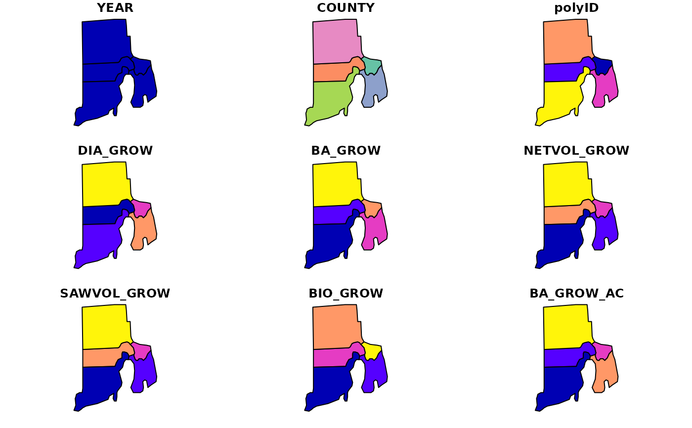
ctSF <- vitalRates(fiaRI_mr,
                   polys = countiesRI,
                   returnSpatial = TRUE)
plot(ctSF) # Plot multiple variables simultaneously
#> Warning: plotting the first 9 out of 24 attributes; use max.plot = 24 to plot all

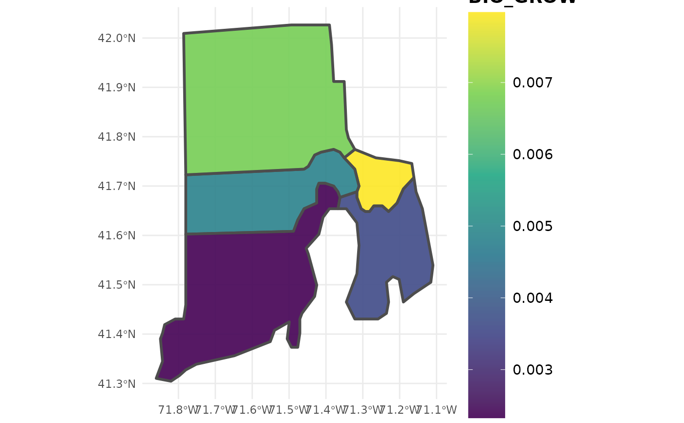
plotFIA(ctSF, BIO_GROW) # Plot of individual tree biomass growth rates

# }